Linear Regression

Linear regression is a statistical technique for drawing a line through a set of data points that “best fits” the data. It is a useful and standard technique for quantifying trends.

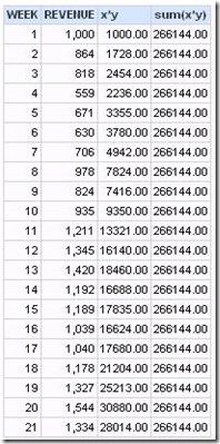
For example, consider the following sample data set, graphed as a simulated dot plot in OBI EE.

Fitting a regression line is a two-step process: finding the slope of the line and finding the y-intercept (where the regression line would cross the y axis).

If you don’t remember the formula for determining the slope from the statistics class you took 10 to 40 years ago (!), you can easily find it with a search on the web. This site has this:

You can calculate this formula directly in Answers. I recommend doing it term by term, using a different calculated column for each term in the formula and then combining terms at the end.

Click on any column in the left panel to get a column to write the first term of the formula in. Here, the column clicked was Revenue.

The first term will be x*y. I label the column headings to correspond to the formula I am building.

Then add another column to continue building the formula, using the Column button in the formula window to pick the x*y column already built. This technique saves a lot of headaches down the road as the formula becomes more complex and you start hunting down unmatched parentheses.

Clicking on x*y gives this formula.

It is useful to look at results for each step along the way. In this case, the results are not what are needed.

So the formula needs to be modified. I added the “by” clause to get the sum for all rows.

As you continue building the regression formula step by step, one of the most problematic seems to be the calculation of the number of rows (N in the formula).

The formula shown here does not work and gives you an error message that is, parenthetically, the answer to the question “What use are logical keys in fact tables?”

State: HY000. Code: 10058. [NQODBC] [SQL_STATE: HY000] [nQSError: 10058] A general error has occurred. [nQSError: 15036] Logical table Facts needs a primary key to support count aggregates on that table. (HY000)

However, instead of creating fact table keys, calculate the count another way. The following formula appears to work (but oddly, as we’ll see, only for a while).

 

Continue building.

Tip: Use the Power() function in your formulas when you can.

Now, the odd thing mentioned above happens. All these columns compute.

However, when you subtract the last column from the next to last to get the denominator in the formula, Answers throws a puzzling error.

State: HY000. Code: 10058. [NQODBC] [SQL_STATE: HY000] [nQSError: 10058] A general error has occurred. [nQSError: 22023] An arithmetic operation is being carried out on a non-numeric type. (HY000)

At least one of the two numbers in the final column is now regarded as non-numeric?

A solution to this seems to be to change the formula for N, which was max(count(rsum(1))). Both max(rsum(1)) or sum(1 by) work.

When you have the numerator(the first column in the following screen shot) and denominator (next to last column) built, calculate the slope.

To plot the regression line, you also need the y intercept. The Criteria tab already has all the terms you need to plug into the intercept formula.

Once you have the slope and intercept, the regression line (values of y vs x) are easily calculated with the formula y=mx+b explained above (m is the slope, b is the y-intercept).

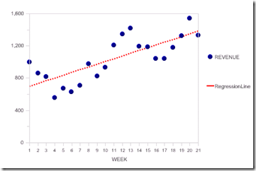
The plot looks like this:

This is a line chart. Revenue is shown with blue round  symbols and a 0 pixel line width. The regression line is a red dotted line with symbols turned off.

Another statistic that is important is the R-squared statistic, which measures how well the regression line fits the data. The formula for R (the correlation coefficient) is:

The Criteria tab already contains the formula for the numerator and several terms of the denominator (circled in this picture).

Build the rest needed for the denominator, then calculate R and finally R-squared.

The final value, 0.58, is the goodness of fit (goodness ranging from 0, bad, to 1, perfect).

At this point all the unneeded columns can be hidden or deleted.

It is always good to translate this into business (i.e. not statistical terms) by renaming things (“Regression” –> “Trend”) and using the narrative view to spell things out as explicitly as possible. Perhaps you can come up with a good business translation for R-square.

Info On the Web About OBIEE

It may be strange to be writing this with the intention of posting to a blog, but I thought someone should step back a minute and issue a few words of warning about information that can be found on the web about Oracle BI EE.

Some of it is downright wrong and will lead you into trouble. Some of it is incomplete and/or not very clear and you will find yourself working hours to figure out how to get the “advice” to actually work. From my experience, the farther away the advice leads you from the “out of the box” product functionality, the more likely either of these outcomes is to occur.

One of the least well-understood aspects of an OBIEE production environment is maintaining web catalogs, particularly merging “development” web cat elements with the production web catalog. Yes, there is an OBIEE utility for doing this, the Catalog Manager. This utility is the “Fredo” of the OBIEE tools. It no doubt does work in certain situations (nothing is impossible), but my experience is that more often than not it does not work – and betrays you, to boot.

The cursory documentation, lack of practical examples, and confusing terminology (what does “archive” do and how does it differ – and it does! – from the “archive” menu choice in the web catalog manager), plus the fact that catalog manager is highly version sensitive (to the third decimal) means using it is either going to work perfectly or it is not going to work at all. There is not much middle ground.

That being the case, it is tempting to believe advice that you don’t need it at all, that “you can copy individual requests, dashboards or whole folders using filesystem copies” as one blogger wrote. In fact, this is the last thing you should do, as you risk corrupting the web catalog permanently. Insidiously, it may not be corruption that will show up immediately – in fact, things may look OK after you do it. However, signs of rot may soon appear: permissions that are wrong and cannot be corrected; catalog manager functionality that no longer works; catalog manager complaints about web cat corruption; the Set Privileges page of the web admin ceases to work. By this time, you may have invested more work in the ailing web catalog, and if there’s a way to recover from this situation, Oracle has not published it. The inner structure of a web catalog remains quite undocumented.

There’s another flavor of this. You may have wished for some functionality in the product which wasn’t there and suddenly one day you read that it actually is via a clever workaround, and it sounds so tempting to try it.

So you settle down to follow someone’s blog about, say, navigating in place, which is feature that many wished that Oracle BI EE had. Yes, once you figure it out (reading the blog makes it seem quite complex -- partly because the blog introduces complexity into the method that really isn’t necessary) and try it, you discover several limitations the blogger forgot to mention (or hadn’t discovered himself). The technique involves creating a narrative view that dynamically constructs a Go URL within an iFrame on the dashboard page. Navigation from this analysis then happens within the iFrame – i.e. on the same dashboard page.  However, there are limitations. If the dashboard employs a non-default style, the results in the iFrame will not match the dashboard. If you use the Style parameter in the URL to change the style to the dashboard style, it will match but then navigation stops working (you are presented with the logon screen during navigation). Passing a parameter from a dashboard prompt works – as long as the parameter does not contain a space. If navigation does work, there’s no way (besides the browser back button) to return. And to get this far, you have to battle the blog’s text itself – which, for example, does not give you the complete text of the URL used in its own example. In the end, you may, like me, decide that the technique is not really ready for prime time.

Another example somewhat in the same vein is advice on constructing dynamic column headers from presentation variables. Again, this is functionality that it would be nice to have. However, when you read the blog, you discover that there are more cautions and limitations than there are side effects listed on your favorite prescription medicine.

Workarounds and functional compromise are part a consultant’s life. Just be careful about what you read on the web. Even very good blogs can give you impractical, wrong, time-draining advice that has not been adequately tested.

Fact-Based Partitioning

One of the questions that comes up over and over again is how to show all periods in a query when facts don’t exist for all periods or how to show all products when facts don’t exist for all products.

To illustrate the problem, I created a database of fictional frosting sales. This is a very simple star schema having a period table, a product table, and a fact table containing weekly sales data for the last eleven weeks of 2003.

One of the frosting products, the “Party” frosting, was only introduced during the week of 11/6, however. Its sales data look like this – with nothing for the weeks in October.

How do you construct the metadata to show zero sales in October for Party frosting?

This is often thought of as a relational database outer join problem, which brings up another question frequently asked: how do you specify an outer join in the metadata?

Quite often, people think of this as a property of the physical join between these tables. However, if you look at the physical join properties in the metadata, you can see that the dialog does not give you any way to specify that the join should be an outer join. Notice that the join type drop down control is not active – it is grayed out.

When we designed OBIEE, we put control over the join type in the business model diagram because it really is a property of the business model – that is, it’s a property of the relationship between the period dimension and the facts. No matter how many period table sources or fact table sources there might be at different levels of granularity (aggregation), the join relationship should be the same within the business model.

So to change the join type, use the business model diagram and change the join type between the logical tables. In the screen shot shown here, I have changed the join type to “Right Outer”. (“Right” is correct in this context since the table having the rows to preserve, the Weeks logical table, is on the right in this dialog).

If you examine the physical SQL after making the change, you can see the outer join being done, with the “right outer join” now translated into a “left outer join” in the SQL since the Weeks table is now “on the left” in the SQL.

SELECT T2382.DESCRIPTION AS c1,
T2388.WEEK AS c2,
sum(T2373.QS) AS c3
FROM
FROSTINGPRODUCTS T2382,
FROSTINGWEEKS T2388 left outer join
FROSTINGFACTS T2373 On T2373.PERIODKEY = T2388.PERIODKEY
WHERE
( T2373.PRODKEY = T2382.PRODKEY AND T2382.DESCRIPTION = 'Party' )
GROUP BY T2382.DESCRIPTION, T2388.WEEK
ORDER BY c1, c2

So does this solve the problem? If you look at the results, you can see that it doesn’t.

Perhaps you might be thinking that you might need to outer join the product table to the fact table, too. But this doesn’t give you the right results, either. Even with full outer joins, the results are still exactly the same.

This is the physical SQL generated by using full outer joins between the dimension tables and the fact table in the business model.

SELECT t2382.DESCRIPTION AS c1
,t2388.week AS c2
,SUM(t2373.qs) AS c3
FROM frostingproducts t2382
FULL OUTER JOIN (frostingweeks t2388
FULL OUTER JOIN frostingfacts t2373
ON t2373.periodkey = t2388.periodkey)
ON t2373.prodkey = t2382.prodkey
WHERE (t2382.DESCRIPTION = 'Party')
GROUP BY
t2382.DESCRIPTION
,t2388.week
ORDER BY c1,c2

It produces these results

.

Let’s think about how to solve this problem in SQL. First calculate the sum of units sold by week for the ‘Party’ frosting. The SQL for that could look like this:

SELECT  
F.PRODKEY
,W.WEEK
,SUM(F.QS) UnitsSold
FROM    
FROSTINGWEEKS W
INNER JOIN FROSTINGFACTS F
ON F.PERIODKEY = W.PERIODKEY
WHERE    F.PRODKEY IN
(SELECT Prodkey
FROM   FROSTINGPRODUCTS
WHERE  Description = 'Party')
GROUP BY F.PRODKEY, W.WEEK

This SQL would produce the familiar results we have already seen.

For the next step, outer join the Products and Weeks table together without using the fact table.

Select P.Description
, P.Prodkey
, W.Week from
frostingproducts P
,frostingweeks W
where P.Description = 'Party'

Then left join the second result set to the first one. In terms of SQL, it would look like this:

WITH D1 AS
(select F.PRODKEY
,W.WEEK
,sum(F.QS) UnitsSold
FROM
FROSTINGWEEKS W inner join
FROSTINGFACTS F On F.PERIODKEY = W.PERIODKEY
WHERE F.PRODKEY IN (SELECT
Prodkey
FROM
FROSTINGPRODUCTS
WHERE
Description = 'Party')
GROUP BY F.PRODKEY, W.WEEK ORDER BY 2),
D2 AS
(Select P.Description, P.Prodkey, W.Week FROM
frostingproducts P
,frostingweeks W
WHERE P.Description = 'Party')
SELECT D2.Description, D2.Week, nvl(D1.UnitsSold,0) UnitsSold
FROM D2 left join D1
on D2.Prodkey = D1.Prodkey
AND D2.Week=D1.Week
ORDER BY 2

An OBIEE business model could be constructed to produce SQL like this. One way to do it would be to join the period and product tables into a single logical dimension table (outer joining the underlying physical tables in the logical table source), then left joining this dimension table to the logical fact table.

Here’s the physical join diagram, with the join between Products and Weeks being a complex join with the condition 1=1.

A single logical table source combines Products and Weeks.

The business model would contain just two logical tables and a single logical join. Note that it is a Left Outer join.

With this metadata, the logical SQL

SELECT Products.DESCRIPTION
, Weeks.WEEK
, FrostingFacts.UnitsSold
FROM Frosting2
WHERE Products.DESCRIPTION = 'Party'

produces this physical SQL

SELECT

T2534.DESCRIPTION AS c1
, T2539.WEEK AS c2
, sum(nvl(T2526.QS , 0)) AS c3
FROM
(FROSTINGPRODUCTS T2534 /* FrostingProducts2 */
full outer join
FROSTINGWEEKS T2539 /* FrostingWeeks2 */ On 1 = 1) left outer join
FROSTINGFACTS T2526 /* FrostingFacts2 */
On T2526.PERIODKEY = T2539.PERIODKEY
AND T2526.PRODKEY = T2534.PRODKEY
WHERE
( T2534.DESCRIPTION = 'Party' )
GROUP BY T2534.DESCRIPTION, T2539.WEEK
ORDER BY c1, c2

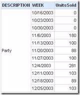
giving the desired results.

(Note on the logical SQL: the columns from the single logical table “FrostingProducts2” have been separated into two presentation layer folders, “Products” and “Weeks”).

However, I don’t recommend this as a solution as you may not always want these results, but now you’ve hard-wired them into the metadata.

A better approach is to take advantage of the concept of “fact-based partitioning”. Fact-based partitioning is a term meaning that facts are stored (“partitioned”) in separate physical tables. These tables are configured as separate logical fact table sources in the metadata. When facts from two fact table sources are included in a query, the BI Server generates SQL with two query blocks and full outer joins the result sets together -- just the behavior we want.

In this case, we need to preserve both the weeks and the products and need a fact that will be returned for all weeks and products specified by the query filter.

I use a one row table to hold this fact. If you’re using Oracle as a database, you can use the virtual table “Dual”. If you’re using SQL Server, you can create a Select statement without a FROM clause to do the same thing (or you can create a one-row table in the database).

Step 1: In the physical layer create a source for the fact that will always be returned. I’ve used a Select statement to create this table:

Step 2: Join this table to the dimension tables with a complex join having the condition 1=1.

Step 3: Add this fact (renamed here as “PreserveDimensions”) as a new logical fact sourced from a new logical table source.

The fact has an aggregation rule of Max. Therefore it will always equal 1.

Step 4: Add this fact to the presentation layer.

Step 5: Create a query with a filter PreserveDimensions = 1 and save this filter. Call it “Preserve Dimensions = True”.

Now to preserve dimensions the user just needs to add this filter to the query. Here’s the query with just a filter on product description:

Now here’s the same query with the Preserve Dimensions filter added:

This query produces physical SQL that has the same form we looked at earlier. It has a query block calculating UnitsSold by Product Description and Week. It has a query block joining the Product Table and the Dimension Table, qualifying the full outer join where Description = ‘Party’.

SELECT
max(T2616.One) AS c1
, T2631.DESCRIPTION AS c2
, T2637.WEEK AS c3
FROM
FROSTINGWEEKS T2637 /* FrostingWeeksFBP */
, FROSTINGPRODUCTS T2631 /* FrostingProductsFBP */
, (SELECT 1 One FROM Dual) T2616
WHERE ( T2631.DESCRIPTION = 'Party' )
GROUP BY
T2631.DESCRIPTION
, T2637.WEEK
HAVING max(T2616.One) = 1

The SQL then outer joins the two result sets together, thereby preserving all the dimension values specified in the query filter.

Note: to display zeros for the weeks where values are NULL, I created a logical column using the ifnull function. In the database, the actual physical column is called QS (i.e. quantity sold). The logical column QS (i.e. Quantity Sold) is mapped directly to this physical column. The logical column UnitsSold is based on the logical column QS.

Now the Answers user can choose whether to display NULLs as zeros or not by selecting the appropriate measure, as well as whether to preserve dimensions or not by clicking on the saved filter.

An alternative to adding the ifnull function in the metadata would be to use it in the column formula on the Criteria tab in Answers.

Note: on versions of OBIEE that included the Time Series functions Ago and ToDate prior to 10.1.3.3.2, this solution would have produced an error since complex joins from a period table source were not allowed. For these versions of OBIEE, the technique described here would have to be modified slightly by altering the Weeks table . Add a column to the Weeks table where all rows have the value of 1. Then join this “key” to the Dual table with a Key/Foreign Key physical join.