[Note: the following discussion is based on OBIEE version 10.1.3.4.0 and Oracle XE version 10G, both running on Windows. The behavior of other versions of OBIEE could be different.]
Typically dimensions have a 1:N relationship to facts. For example, consider a period dimension table at the day level and a fact table containing sales by day and product. For every row in the dimension table there can be many rows in the fact table. However, for every row in the fact table, there is only one associated row in the period table.
However, sometimes things are more complicated. In some cases, each row in the fact table could be associated with many rows in a dimension table. This posting is about modeling this kind of relationship in OBIEE.
Let’s take an example where this could occur. When a customer calls a call center, the customer could discuss many topics. If there is a “topic” dimension (a dimension that lists the topics that could be discussed), there could be be many topics associated with any given call.
For example, consider this Calls table. It contains data for 20 calls. 6 occurred in May, 6 in June, 5 in July, and 3 in August. Each call was one minute long.
There are five topics in the Topics table, four specific topics and a catch-all “Other”.
One way to store which topics were discussed in which call is with the use of a table that associates topics with calls. Such a table can go by several names: “relationship table”, “associative table”, “helper table”, “owner-member table”, or “bridge table” are some terms that have been used. Some of the rows in this table (let’s call it “CallsTopics”) could look like this:
This table tells us that call 1 was entirely about Bills. Call 2 was about the Bills and Other. Call 3 was about Instructions and Other. In our example database, this table has 36 rows.
The physical database schema in this data model looks like this:
This model could be more complex. In real life there could (and should) be a period dimension table associated with the calls. There could also be a customer dimensions, a call center employee dimension, and perhaps other dimensions. In our simple example, however, we will work with just these three tables.
The main facts are the count of calls and the duration of calls. The aggregation rule for “# Calls” is count distinct. The aggregation rule for Duration is sum. Both of these facts come from the Calls table. In most schemas, the fact table is at the N end of all the join relationships that touch it. Notice that this schema is different: the CallTopics table is the one that is at the N end of the joins.
When modeling this in OBIEE, consider that there are two pathways to the Calls table. One logical path is from the Calls table itself used as a dimension table. The other is from the Topics table via the CallTopics table.
One way to model these two pathways is to create two logical fact table sources. One would contain the Calls table alone. The other would contain Calls and CallTopics, as shown in the following screen shot.
The entire business model looks like this.
By the way, the business model diagram shows the normal 1:N relationships between logical dimension tables and logical fact tables in that the logical fact table is at the N end of every logical join that touches it.
In the business model, the two fact table sources can be thought of as being at two different levels of aggregation. With two dimensions, Calls and Topics, the Calls source is at the Total level for Topics.
The other source, “CallsAndTopics”, is at the detail level for the two dimensions.
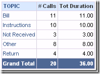
A query for facts by topic using this business model produced these results:
The way to interpret the numbers in the Tot Duration column is that for each topic, this is the sum of the duration of calls that included that topic. In other words, 11 phone calls with a total duration of 11 minutes included the topic of billing. However, the Grand Total of 36 is a more questionable number. Shouldn’t the “Tot Duration” Grand Total be 20?
It turns out that the value shown for the Duration Grand Total depends on the method of aggregation that is being used. The aggregation rule is set in the Edit Column Formula dialog. To begin with, the default aggregation rule is inherited from the aggregation rule set for the column in the metadata. In this case, it is SUM.
Notice what happens when the Server Complex Aggregate rule is used instead.
The use of different aggregation rules resulted in different logical SQL, with REPORT_SUM used when the aggregation rule was “Default” (inherited from SUM) and AGGREGATE when “Server Complex Aggregate”.
The different logical SQL statements resulted in different physical SQL statements.
With REPORT_SUM there were two Select statements to the database (sum call duration and count distinct calls by topic in the first select; count distinct calls overall), with an additional six select statements issued to manipulate the results of the first two queries, including calculating the report sum.
In the case of the AGGREGATE rule, an additional SQL statement was issued to sum the overall duration. This is the query that eliminated the over-counting. Then two additional select statements were used to manipulate the results of the first three queries.
Note that by changing the aggregation rule to server complex aggregate, then opening the column properties dialog and saving as the system-wide default, the AGGREGATE function will become the default aggregation rule in the future. (Re-read the warning about version-specific behavior at the beginning of this post.)
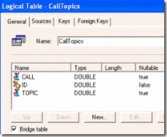
Another way to model this is to take the CALLTOPICS table out of the fact table source and create a new logical table that acts as a “bridge table” between the Topics table and the Calls table. Note that the Bridge table property is checked here.
The business model now looks like this.
The default results are shown here.
The logical SQL issued uses the AGGREGATE rule by default.
Switching the aggregation rule in the column formula dialog to SUM changes the results and the logical SQL.
Summary: In data models such as this where you have the possibility of double counting results in totals, be aware that the totals will depend on the aggregation rules set for the measures on the Criteria tab.
Default behavior depends on how the business model is configured and which aggregation rule is being used as the default.


